Linear regression is one of the simplest yet powerful algorithms in machine learning. It serves as the foundation for more complex models and is widely used in predictive analysis, trend forecasting, and understanding relationships between variables. This blog post dives into the concepts, mathematical foundations, applications, and practical implementation of linear regression, complete with schematic diagrams for better comprehension.
What is Linear Regression?
Linear regression is a supervised learning algorithm used to predict a continuous target variable (dependent variable) based on one or more predictor variables (independent variables). The goal is to find a linear relationship between the input features and the target variable by fitting a straight line to the data points.
Mathematically, the relationship is represented as:$$y = w_1 x + b + \epsilon$$
Where:
- \(y\): Target variable
- \(x\): Input feature
- \(b\): Intercept of the line (bias term)
- \(w_1\): Slope of the line (weight)
- \(\epsilon\): Error term
Types of Linear Regression
Simple Linear Regression
Simple linear regression involves a single independent variable and models a straight-line relationship with the dependent variable. The equation is represented as:$$y = w_1 x + b + \epsilon$$
where \(x\) is the single independent variable.
Multiple Linear Regression
Multiple linear regression extends the concept to multiple independent variables, with the equation:$$y = w_1 x_1 + w_2 x_2 + \dots + w_n x_n + b + \epsilon$$
where:
- \(x_1, x_2, \dots, x_n\): Independent variables
- \(w_1, w_2, \dots, w_n\): Corresponding weights (coefficients) for each independent variable
- \(b\): Intercept (bias term)
- \(\epsilon\): Error term
Mathematical Foundation
- Cost Function
The cost function measures how well the line fits the data. Linear regression uses the Mean Squared Error (MSE) as the cost function:$$J(w, b) = \frac{1}{2m} \sum_{i=1}^{m} \left( \hat{y}_i – y_i \right)^2$$Where:- \(\hat{y}_i\): Predicted value for the \(i\)-th data point
- \(y_i\): Actual value for the \(i\)-th data point
- \(m\): Number of data points
- Gradient Descent
Gradient descent is an optimization algorithm used to minimize the cost function. The parameters are updated iteratively:$$bw_j := w_j – \alpha \frac{\partial J(w, b)}{\partial w_j}, \quad b := b – \alpha \frac{\partial J(w, b)}{\partial b}$$Where:- \(\alpha\): Learning rate
- \(\frac{\partial J(w, b)}{\partial w_j}\): Partial derivative of the cost function with respect to \(w_j\)
- \(\frac{\partial J(w, b)}{\partial b}\): Partial derivative of the cost function with respect to \(b\)
Visual Representation
Data Points and Line Fitting
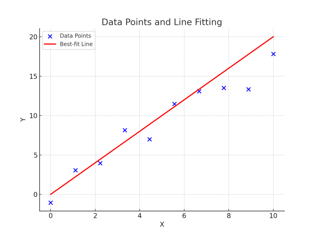
Below is a schematic diagram illustrating data points and the fitted regression line:

The blue dots represent the data points, while the red line is the best-fit line minimizing the cost function.
Error Visualization

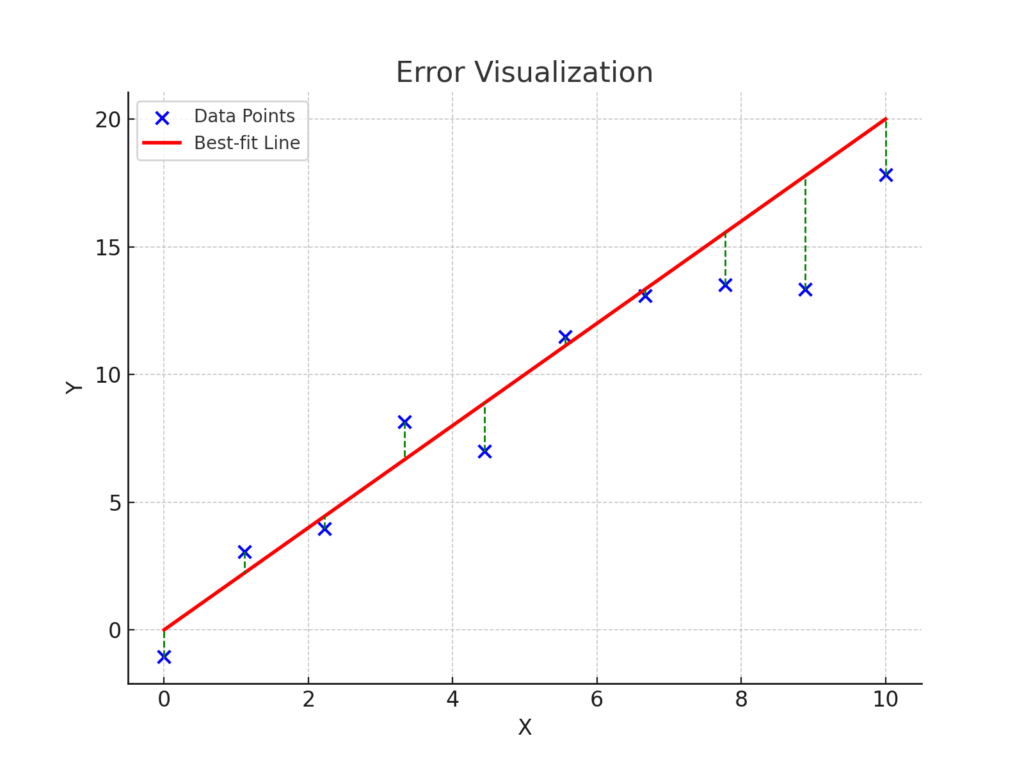
The vertical lines between the data points and the regression line show the residual errors (\(y_i – \hat{y}_i\)). These residuals represent the differences between the actual values and the predicted values. Minimizing these errors is the objective of the regression process.
Applications of Linear Regression
- Predictive Modeling: Forecasting sales, stock prices, and other continuous variables.
- Trend Analysis: Identifying trends in data, such as growth or decline.
- Risk Assessment: Evaluating relationships between risk factors and outcomes in fields like insurance and healthcare.
- Econometrics: Analyzing economic relationships, such as the impact of interest rates on investments.
Implementation in Python
Here is a simple implementation of linear regression using Python and Scikit-Learn:
import numpy as np
import matplotlib.pyplot as plt
from sklearn.linear_model import LinearRegression
from sklearn.model_selection import train_test_split

# Sample Data
X = np.array([1, 2, 3, 4, 5]).reshape(-1, 1)
y = np.array([2.2, 2.8, 4.5, 4.9, 5.7])

# Splitting Data
X_train, X_test, y_train, y_test = train_test_split(X, y, test_size=0.2, random_state=42)

# Model Training
model = LinearRegression()
model.fit(X_train, y_train)

# Predictions
y_pred = model.predict(X_test)

# Visualization
plt.scatter(X, y, color='blue', label='Data Points')
plt.plot(X, model.predict(X), color='red', label='Regression Line')
plt.legend()
plt.show()
Conclusion
Linear regression is an indispensable tool in the data scientist’s arsenal. Its simplicity, interpretability, and effectiveness make it a popular choice for solving real-world problems. By understanding the theory and mathematics behind it, you can better utilize this algorithm for predictive modeling and data analysis.
Whether you are a beginner or an experienced practitioner, mastering linear regression lays a strong foundation for delving into advanced machine learning techniques.