When it comes to machine learning, few concepts are as foundational and transformative as gradient descent. This optimization algorithm lies at the heart of many machine learning models, enabling systems to learn from data and improve their predictions over time. In this blog post, we delve into the mechanics of gradient descent, focusing on its application in linear regression. We’ll explore its principles, mathematical foundation, and practical implementation, making it approachable for enthusiasts and professionals alike.
What is Gradient Descent?
Gradient descent is an iterative optimization algorithm used to minimize a loss function. In the context of linear regression, the loss function quantifies how far off the predictions of our model are from the actual target values. By minimizing this loss, we improve the model’s accuracy.
The essence of gradient descent lies in its name: it uses the gradient (or slope) of the loss function to “descend” to its minimum value. Think of it as a hiker trying to reach the lowest point in a valley, guided by the steepness of the terrain.
The Role of Gradient Descent in Linear Regression
Linear regression models the relationship between input features and a continuous target variable by fitting a straight line. Mathematically, the relationship can be expressed as:$$y = \theta_0 + \theta_1 x$$
Here:
- \(y\): Predicted target value
- \(\theta_0\): Intercept (bias)
- \(\theta_1\): Slope (weight)
- \(x\): Input feature

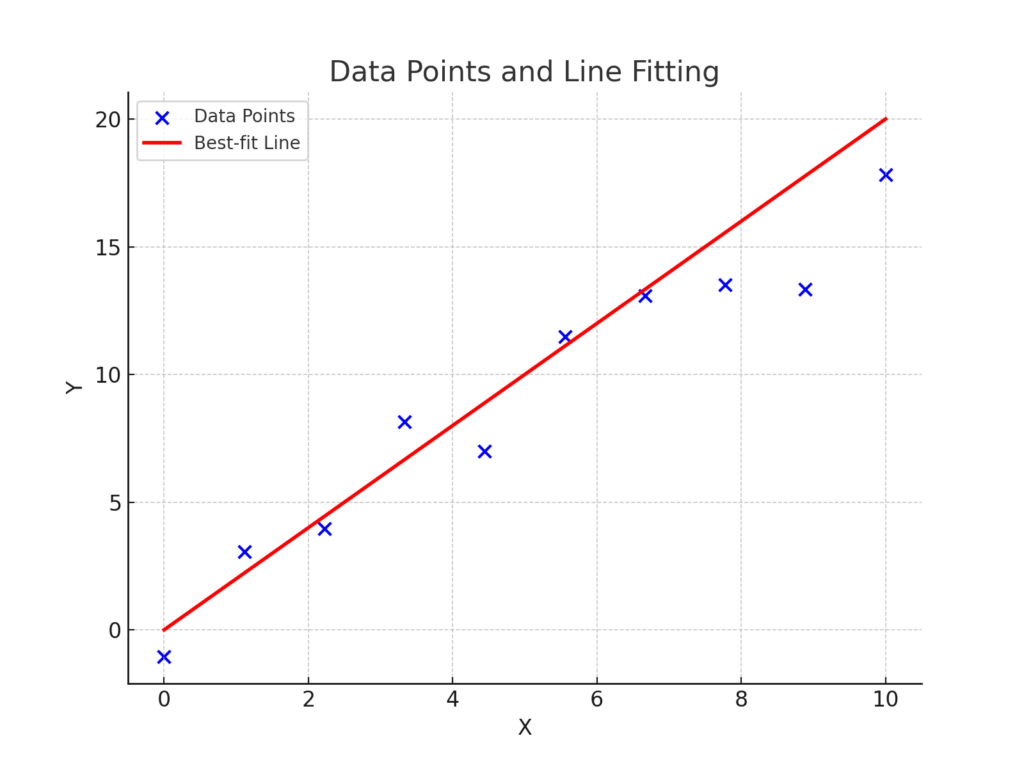
The blue dots represent the data points. The goal is to find the best-fit line (the red line) minimizing the cost function. In other words finding the optimal parameters (\(\theta_0\) and \(\theta_1\)) that minimize the error between predicted and actual values. The error is quantified using the cost function \(J(\theta_0, \theta_1)\), defined as:$$J(\theta_0, \theta_1) = J(\theta) = \frac{1}{2m} \sum_{i=1}^{m} \left( \hat{y}_i – y_i \right)^2$$
where:
- \(m\): Number of data points
- \(\hat{y}_i = \theta_0 + \theta_0 x_i\): Predicted target value for the \(i\)-th data point
- \(y_i\): Actual target value for the \(i\)-th data point
Gradient descent is employed to iteratively adjust the parameters \(\theta_0\) (bias) and \(\theta_1\) (weight) to minimize \(J(\theta_0, \theta_1)\) or \(J(\theta)\). This optimization algorithm updates the parameters by computing the gradient of the cost function with respect to each parameter and moving in the direction of steepest descent. The update rules for the parameters are given by:$$\theta_0 = \theta_0 – \alpha \frac{\partial J(\theta_0, \theta_1)}{\partial \theta_0}$$ $$\theta_1 = \theta_1 – \alpha \frac{\partial J(\theta_0, \theta_1)}{\partial \theta_1}$$
Here, \(\alpha\) is the learning rate, which controls the step size for each iteration. By repeating this process, gradient descent ensures convergence toward the optimal values of www and \(b\), thus fitting the best line to the data.
The Gradient Descent Process
Gradient descent updates the parameters iteratively to reduce the loss. The update rule for each parameter is:$$\theta_j \leftarrow \theta_j – \alpha \frac{\partial J(\theta)}{\partial \theta_j}$$
Where:
- \(\alpha\): Learning rate, controlling the step size of each update
- \(\frac{\partial J(\theta)}{\partial \theta_j}\): Partial derivative of the loss function with respect to \(\theta_j\)
For linear regression, the cost function is the Mean Squared Error (MSE):$$J(\theta) = \frac{1}{2m} \sum_{i=1}^{m} \left( \hat{y}_i – y_i \right)^2$$
The partial derivatives of the cost function with respect to \(\theta_0\) (intercept) and \(\theta_1\) (slope) are derived as follows:
- Partial derivative with respect to \(\theta_0\):
$$\frac{\partial J(\theta)}{\partial \theta_0} = \frac{1}{m} \sum_{i=1}^{m} \left( \hat{y}_i – y_i \right)$$
- Partial derivative with respect to \(\theta_1\):
$$\frac{\partial J(\theta)}{\partial \theta_1} = \frac{1}{m} \sum_{i=1}^{m} \left( \hat{y}_i – y_i \right) x_i$$
Here:
- \(m\): Number of training examples
- \(\hat{y}_i = \theta_0 + \theta_1 x_i\): Predicted target value for the \(i\)-th example
- \(y_i\): Actual target value for the \(i\)-th example
- \(x_i\): Input feature for the \(i\)-th example
How these derivatives are computed:
- For \(\frac{\partial J(\theta)}{\partial \theta_0}\), the term \(\left( \hat{y}_i – y_i \right)\) measures the residual error for each data point, and the gradient is the average of these errors across all data points. This controls how much to adjust \(\theta_0\).
- For \(\frac{\partial J(\theta)}{\partial \theta_1}\), the term \(\left( \hat{y}_i – y_i \right) x_i\) measures the error scaled by the input feature \(x_i\). This determines how much \(\theta_1\) should be adjusted to reduce the error for each data point.
By iteratively updating \(\theta_0\) and \(\theta_1\) using these gradients, the algorithm minimizes the loss function, converging to the optimal parameters that best fit the data.
Partial Derivative with Respect to \(\theta_0\) (Intercept)
We aim to compute:$$\frac{\partial J(\theta)}{\partial \theta_0}$$
Substitute \(\hat{y}_i = \theta_0 + \theta_1 x_i\) into \(J(\theta)\):$$J(\theta) = \frac{1}{2m} \sum_{i=1}^{m} \left( (\theta_0 + \theta_1 x_i) – y_i \right)^2$$
Let \(e_i = \hat{y}_i – y_i = (\theta_0 + \theta_1 x_i) – y_i\), the error for the \(i\)-th data point. Then:$$J(\theta) = \frac{1}{2m} \sum_{i=1}^{m} e_i^2$$
Take the derivative of \(J(\theta)\) with respect to \(\theta_0\):$$\frac{\partial J(\theta)}{\partial \theta_0} = \frac{\partial}{\partial \theta_0} \left( \frac{1}{2m} \sum_{i=1}^{m} e_i^2 \right)$$
Since \(e_i = (\theta_0 + \theta_1 x_i – y_i)\), the derivative of \(e_i^2\) with respect to \(\theta_0\) is:$$\frac{\partial e_i^2}{\partial \theta_0} = 2 e_i \cdot \frac{\partial e_i}{\partial \theta_0}$$
Here, \(\frac{\partial e_i}{\partial \theta_0} = 1\), because \(\theta_0\) appears linearly in \(e_i\). Thus:$$\frac{\partial e_i^2}{\partial \theta_0} = 2 e_i$$
Substitute this back into the derivative:$$\frac{\partial J(\theta)}{\partial \theta_0} = \frac{1}{2m} \sum_{i=1}^{m} 2 e_i \cdot 1 = \frac{1}{m} \sum_{i=1}^{m} e_i$$
Replace \(e_i = (\hat{y}_i – y_i)\):$$\frac{\partial J(\theta)}{\partial \theta_0} = \frac{1}{m} \sum_{i=1}^{m} \left( \hat{y}_i – y_i \right)$$
Partial Derivative with Respect to \(\theta_1\) (Slope)
Now, compute:$$\frac{\partial J(\theta)}{\partial \theta_1}$$
Using the same cost function \(J(\theta)\):$$J(\theta) = \frac{1}{2m} \sum_{i=1}^{m} \left( (\theta_0 + \theta_1 x_i) – y_i \right)^2$$
Take the derivative of \(J(\theta)\) with respect to \(\theta_1\):$$\frac{\partial J(\theta)}{\partial \theta_1} = \frac{\partial}{\partial \theta_1} \left( \frac{1}{2m} \sum_{i=1}^{m} e_i^2 \right)$$
As before, \(\frac{\partial e_i^2}{\partial \theta_1} = 2 e_i \cdot \frac{\partial e_i}{\partial \theta_1}\). Now, compute \(\frac{\partial e_i}{\partial \theta_1}\):$$e_i = (\theta_0 + \theta_1 x_i – y_i)$$ $$\frac{\partial e_i}{\partial \theta_1} = x_i$$
Thus:$$\frac{\partial e_i^2}{\partial \theta_1} = 2 e_i $$
Substitute this back into the derivative:$$\frac{\partial J(\theta)}{\partial \theta_1} = \frac{1}{2m} \sum_{i=1}^{m} 2 e_i x_i$$ $$\frac{\partial J(\theta)}{\partial \theta_1} = \frac{1}{m} \sum_{i=1}^{m} \left( \hat{y}_i – y_i \right) x_i$$
Visualizing Gradient Descent
3D Visualizing of Gradient Descent

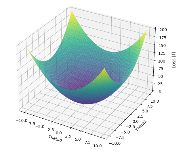
To better understand the process, consider a 3D plot where:
- The x- and y-axes represent parameters \(\theta_0\) and \(\theta_1\).
- The z-axis represents the value of the loss function \(J(\theta_0, \theta_1)\).
The surface represents the behavior of the loss function for different values of \(\theta_0\) and \(\theta_1\). Gradient descent can be visualized as a ball rolling down the slope of this surface, eventually settling at the lowest point, which corresponds to the global minimum.
The trajectory of the ball is influenced by the learning rate (\(\alpha\)):
- A large \(\alpha\) may cause the ball to overshoot the minimum, resulting in divergence or oscillation around the minimum.
- A small \(\alpha\) ensures stability but results in slow convergence, making the process computationally expensive.
Contours of Gradient Descent

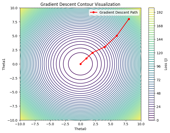
Another way to visualize gradient descent is through a 2D contour plot. In this view:
- The contour lines represent constant values of the loss function.
- The goal is to reach the center of the innermost contour, which represents the global minimum.
At each iteration, gradient descent computes the gradient of the loss function and updates the parameters, effectively moving the point closer to the minimum. The path traced by these updates resembles a series of steps that spiral or zigzag toward the center, depending on the learning rate and the shape of the loss function surface.
By adjusting the learning rate and monitoring convergence, gradient descent ensures efficient optimization of the parameters for linear regression or other machine learning models.
Practical Implementation in Python
Here’s a simple implementation of gradient descent for linear regression:
import numpy as np

# Hypothetical dataset
X = np.array([1, 2, 3, 4, 5])  # Input feature
y = np.array([1.2, 2.4, 3.1, 4.3, 5.0])  # Target variable

# Parameters
m = len(X)
theta_0, theta_1 = 0, 0  # Initial values
alpha = 0.01  # Learning rate
iterations = 1000

# Gradient Descent
for _ in range(iterations):
    predictions = theta_0 + theta_1 * X
    error = predictions - y

    # Compute gradients
    gradient_theta_0 = (1 / m) * np.sum(error)
    gradient_theta_1 = (1 / m) * np.sum(error * X)

    # Update parameters
    theta_0 -= alpha * gradient_theta_0
    theta_1 -= alpha * gradient_theta_1

print(f"Optimized parameters: theta_0 = {theta_0}, theta_1 = {theta_1}")
Key Takeaways
- Gradient descent is the backbone of optimization in machine learning.
- Its iterative nature ensures it can handle complex loss functions.
- The choice of learning rate significantly influences its efficiency and convergence.
Understanding gradient descent deepens your appreciation of how machine learning models “learn.” While linear regression offers a relatively simple use case, the same principles extend to more complex algorithms and architectures. Mastering this foundational tool opens the door to unlocking the full potential of machine learning.
Final Thoughts
As the demand for predictive models grows, grasping the inner workings of optimization techniques like gradient descent becomes essential for practitioners. Whether you’re fine-tuning a linear regression model or training deep neural networks, the knowledge of gradient descent is your guiding compass on the journey to data-driven insights.