Understanding Gradient Descent in AI/ML

In the ever-evolving landscape of artificial intelligence and machine learning, Gradient Descent stands out as one of the most pivotal optimization algorithms. From training linear regression models to fine-tuning complex neural networks, it forms the foundation of how machines learn from data. By iteratively adjusting model parameters to minimize errors, Gradient Descent enables AI systems to make better predictions and decisions over time.

This post dives deep into the concept of Gradient Descent, unraveling its mathematics, types, challenges, and applications, all accompanied by illustrative examples and diagrams for clarity.

What is Gradient Descent?

Gradient Descent is an iterative optimization algorithm used to minimize a cost (or loss) function. It adjusts model parameters (weights and biases) step-by-step to reduce the error in predictions.

Imagine standing on a mountain in the dark and trying to reach the lowest valley. You use a flashlight to determine the steepest downward path and take small steps in that direction. This process is akin to gradient descent.

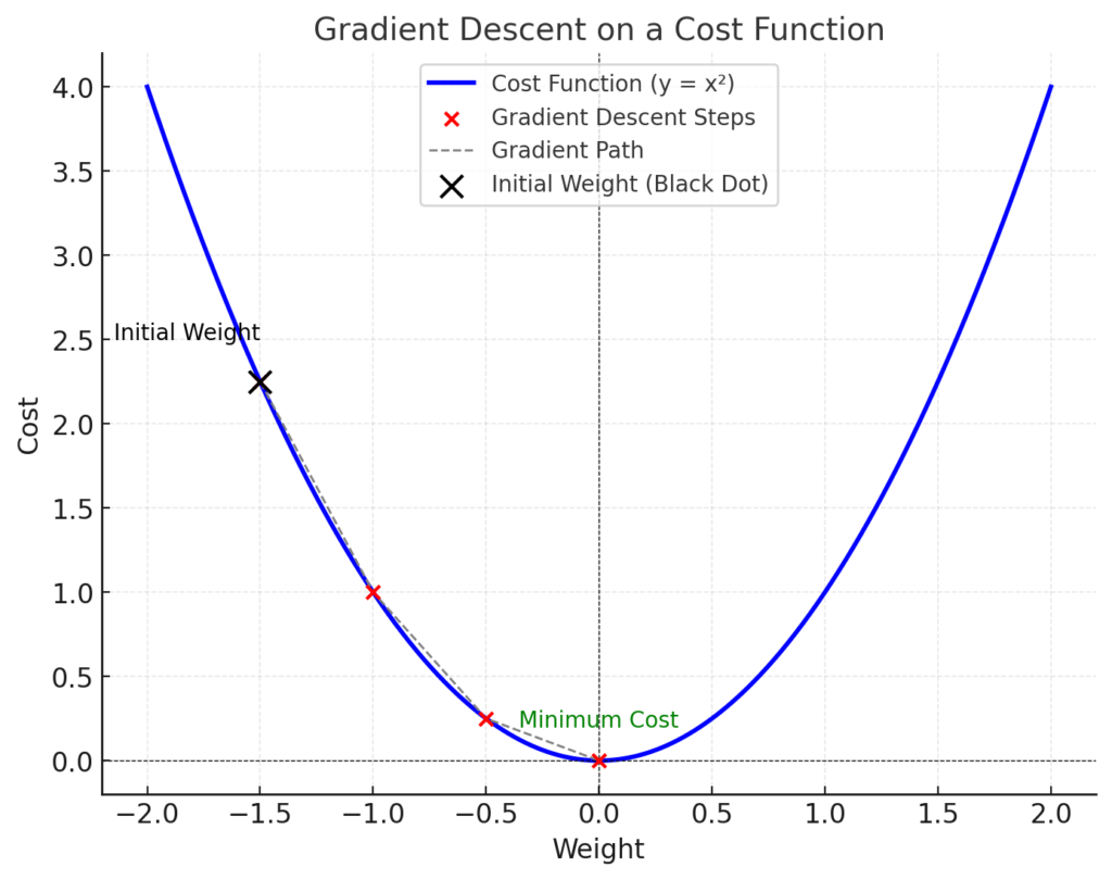
In the diagram above:

• The parabola represents the cost function.
• The black dot indicates the initial weight.
• The gradient (dashed line) shows the direction of the steepest ascent, which we avoid by moving in the opposite direction.
• The red dots show incremental steps taken toward the minimum cost, where the model achieves optimal performance.

Mathematics Behind Gradient Descent

Gradient Descent is a fundamental optimization algorithm used in machine learning and deep learning to minimize a cost or loss function. Mathematically, given a function \(f(\mathbf{\theta})\), where \(\mathbf{\theta}\) represents the parameters to optimize, gradient descent iteratively updates \(\mathbf{\theta}\) in the direction of the negative gradient of \(f(\mathbf{\theta})\). The update rule is given by:$$\mathbf{\theta}_{t+1} = \mathbf{\theta}_t – \eta \nabla f(\mathbf{\theta}_t),$$

where \(\eta\) is the learning rate, a small positive scalar that controls the step size, and \(\nabla f(\mathbf{\theta}_t)\) is the gradient of \(f(\mathbf{\theta})\) with respect to \(\mathbf{\theta}\) at iteration \(t\). The gradient \(\nabla f(\mathbf{\theta}_t)\) is a vector of partial derivatives:$$\nabla f(\mathbf{\theta}) = \left[ \frac{\partial f}{\partial \theta_1}, \frac{\partial f}{\partial \theta_2}, \ldots, \frac{\partial f}{\partial \theta_n} \right]^T.$$

This process iteratively reduces the value of the function \(f(\mathbf{\theta})\) until convergence, ideally reaching a local or global minimum. For convex functions, gradient descent guarantees convergence to the global minimum, while for non-convex functions, it may converge to a local minimum or saddle point.

Types of Gradient Descent

1. Batch Gradient Descent:
   • Uses the entire dataset to compute the gradient.
   • Slower but more stable.
   • Not suitable for very large datasets.
2. Stochastic Gradient Descent (SGD):
   • Uses a single data point to compute the gradient.
   • Faster but introduces noise in the updates.
3. Mini-batch Gradient Descent:
   • A compromise between batch and SGD.
   • Divides the dataset into smaller batches.

Example: Gradient Descent for Linear Regression

Gradient Descent is often used to minimize the cost function for linear regression. For example, in a simple linear regression model, the hypothesis is represented as $$h(x) = \theta_1 x + \theta_2​,$$ where \(\theta_1\)​ (slope) and \(\theta_2\)​ (intercept) are the parameters to be learned.

The algorithm starts by initializing \(\theta_1\)​ and \(\theta_2\)​ with random values and iteratively updates them to minimize the cost function, typically the Mean Squared Error (MSE). Using the update rules $$\theta_1 := \theta_1 – \alpha \frac{\partial J}{\partial \theta_1}$$​ and $$\theta_2 := \theta_2 – \alpha \frac{\partial J}{\partial \theta_2},$$​ where \(J\) is the cost function and \(\alpha\) is the learning rate, the algorithm adjusts the parameters in the direction of steepest descent.

Over time, gradient descent converges to the optimal values of \(\theta_1\)​ and \(\theta_2\)​, resulting in a line that minimizes the error between predicted and actual values.

Python Implementation

Here is a Python implementation of gradient descent for minimizing a quadratic cost function. We’ll explain each part of the code and provide the output for better understanding.

We will use the example of finding the minimum of a simple quadratic function \(f(x) = x^2\).

import numpy as np
import matplotlib.pyplot as plt

# Gradient Descent Implementation
def gradient_descent(start_x, learning_rate, iterations):
    x = start_x  # Starting point
    history = []  # To store the values of x for visualization
    
    for i in range(iterations):
        gradient = 2 * x  # Derivative of f(x) = x^2
        x = x - learning_rate * gradient
        history.append(x)
        print(f"Iteration {i+1}: x = {x:.4f}, Gradient = {gradient:.4f}")
    
    return x, history

# Parameters
start_x = 10  # Initial value of x
learning_rate = 0.1  # Step size
iterations = 20  # Number of iterations

# Run gradient descent
final_x, history = gradient_descent(start_x, learning_rate, iterations)

# Output the final result
print(f"\nFinal result: x = {final_x:.4f}")

# Plotting the results
x_vals = np.linspace(-12, 12, 100)
y_vals = x_vals**2

plt.figure(figsize=(10, 6))
plt.plot(x_vals, y_vals, label="f(x) = x^2", color="blue")
plt.scatter(history, [x**2 for x in history], color="red", label="Steps")
plt.title("Gradient Descent Optimization")
plt.xlabel("x")
plt.ylabel("f(x)")
plt.legend()
plt.grid()
plt.show()

Explanation

Quadratic Function:
The function \(f(x) = x^2\) has a minimum at \(x = 0\). Its derivative is \(f'(x) = 2x\), which we use to compute the gradient.

Algorithm:

• Start with an initial value for xxx (e.g., start_x = 10).
• Compute the gradient using \(2x\).
• Update xxx by moving it in the opposite direction of the gradient: \(x_{\text{new}} = x – \text{learning_rate} \times \text{gradient}\)

Parameters:

• learning_rate: Controls how big a step is taken in each iteration.
• iterations: Number of times the update is performed.

Example Output

Iteration 1: x = 8.0000, Gradient = 20.0000
Iteration 2: x = 6.4000, Gradient = 16.0000
Iteration 3: x = 5.1200, Gradient = 12.8000
...
Iteration 20: x = 0.0118, Gradient = 0.0235

Final result: x = 0.0118

Visualization:

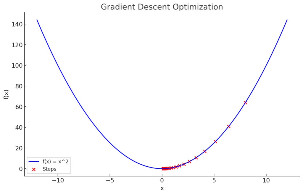
Here’s the plot for the gradient descent process. The blue curve represents the function \(f(x) = x^2\), and the red points show the steps taken by the algorithm toward the minimum at \(x = 0\).

Challenges in Gradient Descent

1. Choosing the Learning Rate:
   • A very small learning rate makes convergence slow.
   • A large learning rate may overshoot the minimum or cause divergence.
2. Local Minima:
   • Some cost functions have multiple minima.
   • Advanced techniques like momentum and Adam optimizer help overcome this.
3. Vanishing and Exploding Gradients:
   • In deep learning, gradients can become too small or too large, making training unstable.

Conclusion

Gradient Descent is a cornerstone of AI/ML, enabling models to learn from data by iteratively minimizing error. Understanding its mechanism, challenges, and enhancements is essential for anyone diving into the world of machine learning. With this knowledge, you can now appreciate the inner workings of optimization in modern AI applications.

If you also want to contribute, click here.